MEDIAN IFs and QUARTILE IFs in MS Excel
Hello friends!! today we’ll be learning how to calculate Median and Quartile values with multiple conditions. I’ve attached the Excel workbook for download and reuse. So it is MEDIAN IFs and QUARTILE IFs but there is no direct formula we’ll create one.
There are few formulas available to aggregate for multiple conditions like IFS, AVERAGEIFS, COUNTIFS, MAXIFS, MINIFS, SUMIFS etc. but there is no inbuilt formula to calculate Median or Quartile with multiple conditions. We can use the same logic to aggregate values on other level.
Sample Data – Here I’ve sample data for electronic gadgets and with brand and some values(table below)
| Category | Brand | Quantity |
| Accesories | Adventure Bags | 9311 |
| Accesories | Adventure Bags | 17399 |
| Accesories | Adventure Bags | 18584 |
| Accesories | Adventure Bags | 6642 |
| Accesories | Adventure Bags | 9844 |
| Accesories | Adventure Bags | 13083 |
| Accesories | Adventure Bags | 18457 |
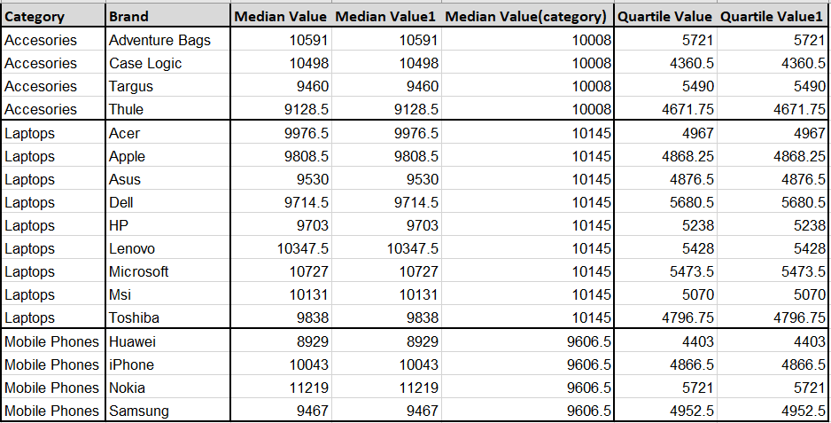
Here I want to calculate the median and 1st Quartile of each category-brand combination or any combination as shown below

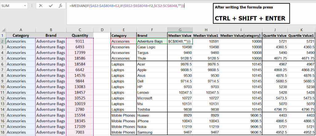
I’ve calculated the median and quartile using array formula
MEDIANIFs
Column G
=MEDIAN(IF(CriteriaRange1 = Criteria1,IF(CriteriaRange2 = Criteria2,Median Value Range,"")))
=MEDIAN(IF($A$2:$A$8048=E2,IF($B$2:$B$8048=F2,$C$2:$C$8048,"")))
Press CTRL + SHIFT + ENTER to activate array formula

Column H – Alternatively you can use the following formula since AND/OR function doesn’t work in array formula so we have to use * for AND, + for OR
=MEDIAN(IF((CriteriaRange1 = Criteria1)(CriteriaRange2 = Criteria2),Median Value Range,""))
=MEDIAN(IF(($A$2:$A$8048=E2)($B$2:$B$8048=F2),$C$2:$C$8048,""))
Press CTRL + SHIFT + ENTER to activate array formula
Column G and Column H returns the same value with slight change in the formula
QUARTILEIFs
Similarly I’ve used array formula to calculate the 1st quartile or 25th percentile.
Column J
=QUARTILE(IF((CriteriaRange1=Criteria1),IF((CriteriaRange2=Criteria2),QuartileValue Range),""),N)
N ranges from 0 t0 4, 0 min value, 1- 1st quartile and so on..
=QUARTILE(IF(($A$2:$A$8048=E2),IF(($B$2:$B$8048=F2),$C$2:$C$8048),"
"),1)
Press CTRL + SHIFT + ENTER to activate array formula
Column K
=QUARTILE(IF((CriteriaRange1 = Criteria1)(CriteriaRange2 = Criteria2),Quartile Value Range),N)
N ranges from 0 t0 4, 0 min value, 1- 1st quartile and so on..
=QUARTILE(IF(($A$2:$A$8048=E2)($B$2:$B$8048=F2),$C$2:$C$8048),1)
Press CTRL + SHIFT + ENTER to activate array formula
Download the Excel Workbook here
Keep visiting Analytics Tuts for more tutorials.
Thanks for reading! Comment your suggestions and queries
